Practical 7

Import Data and pacakge

install.packages(pkgs="http://www.karlin.mff.cuni.cz/~hlavka/sms2/SMSdata_1.0.tar.gz", repos=NULL, type="source")

## Installation du package dans 'C:/Users/guill/OneDrive/Documents/R/win-library/4.1'
## (car 'lib' n'est pas spécifié)

library(SMSdata)
data(food)
library("FactoMineR")

## Warning: le package 'FactoMineR' a été compilé avec la version R 4.1.3

library("factoextra")

## Warning: le package 'factoextra' a été compilé avec la version R 4.1.3

## Le chargement a nécessité le package : ggplot2

## Welcome! Want to learn more? See two factoextra-related books at https://goo.gl/ve3WBa

library("qgraph")

## Warning: le package 'qgraph' a été compilé avec la version R 4.1.3

library(corrplot)

## corrplot 0.92 loaded

library(tidyverse)

## Warning: le package 'tidyverse' a été compilé avec la version R 4.1.3

## -- Attaching packages --------------------------------------- tidyverse 1.3.1 --

## v tibble  3.1.6     v dplyr   1.0.8
## v tidyr   1.2.0     v stringr 1.4.0
## v readr   2.1.2     v forcats 0.5.1
## v purrr   0.3.4

## Warning: le package 'readr' a été compilé avec la version R 4.1.3

## Warning: le package 'forcats' a été compilé avec la version R 4.1.3

## -- Conflicts ------------------------------------------ tidyverse_conflicts() --
## x dplyr::filter() masks stats::filter()
## x dplyr::lag()    masks stats::lag()

library(psych)

## Warning: le package 'psych' a été compilé avec la version R 4.1.3

## 
## Attachement du package : 'psych'

## Les objets suivants sont masqués depuis 'package:ggplot2':
## 
##     %+%, alpha

Evaluate the correlation matrix

library(RcmdrMisc)

## Warning: le package 'RcmdrMisc' a été compilé avec la version R 4.1.3

## Le chargement a nécessité le package : car

## Le chargement a nécessité le package : carData

## 
## Attachement du package : 'car'

## L'objet suivant est masqué depuis 'package:psych':
## 
##     logit

## L'objet suivant est masqué depuis 'package:dplyr':
## 
##     recode

## L'objet suivant est masqué depuis 'package:purrr':
## 
##     some

## Le chargement a nécessité le package : sandwich

## Warning: le package 'sandwich' a été compilé avec la version R 4.1.3

## 
## Attachement du package : 'RcmdrMisc'

## L'objet suivant est masqué depuis 'package:psych':
## 
##     reliability

rcorr.adjust(food) # This function is build into R Commander.

## 
##  Pearson correlations:
##             bread vegetables  fruits    meat poultry   milk    wine
## bread      1.0000     0.5931  0.1961  0.3213  0.2480 0.8556  0.3038
## vegetables 0.5931     1.0000  0.8563  0.8811  0.8268 0.6628 -0.3565
## fruits     0.1961     0.8563  1.0000  0.9595  0.9255 0.3322 -0.4863
## meat       0.3213     0.8811  0.9595  1.0000  0.9818 0.3746 -0.4372
## poultry    0.2480     0.8268  0.9255  0.9818  1.0000 0.2329 -0.4002
## milk       0.8556     0.6628  0.3322  0.3746  0.2329 1.0000  0.0069
## wine       0.3038    -0.3565 -0.4863 -0.4372 -0.4002 0.0069  1.0000
## 
##  Number of observations: 12 
## 
##  Pairwise two-sided p-values:
##            bread  vegetables fruits meat   poultry milk   wine  
## bread             0.0421     0.5412 0.3086 0.4370  0.0004 0.3371
## vegetables 0.0421            0.0004 0.0002 0.0009  0.0188 0.2554
## fruits     0.5412 0.0004            <.0001 <.0001  0.2915 0.1089
## meat       0.3086 0.0002     <.0001        <.0001  0.2303 0.1552
## poultry    0.4370 0.0009     <.0001 <.0001         0.4663 0.1974
## milk       0.0004 0.0188     0.2915 0.2303 0.4663         0.9831
## wine       0.3371 0.2554     0.1089 0.1552 0.1974  0.9831       
## 
##  Adjusted p-values (Holm's method)
##            bread  vegetables fruits meat   poultry milk   wine  
## bread             0.5471     1.0000 1.0000 1.0000  0.0064 1.0000
## vegetables 0.5471            0.0064 0.0028 0.0137  0.2635 1.0000
## fruits     1.0000 0.0064            <.0001 0.0003  1.0000 1.0000
## meat       1.0000 0.0028     <.0001        <.0001  1.0000 1.0000
## poultry    1.0000 0.0137     0.0003 <.0001         1.0000 1.0000
## milk       0.0064 0.2635     1.0000 1.0000 1.0000         1.0000
## wine       1.0000 1.0000     1.0000 1.0000 1.0000  1.0000

KMO Test (Kaiser-Meyer-Olkin)

library(psych)

KMO(food)

## Kaiser-Meyer-Olkin factor adequacy
## Call: KMO(r = food)
## Overall MSA =  0.46
## MSA for each item = 
##      bread vegetables     fruits       meat    poultry       milk       wine 
##       0.55       0.51       0.50       0.48       0.46       0.39       0.25

• 0.00 to 0.49 unacceptable
• 0.50 to 0.59 miserable

The Kaiser–Meyer–Olkin (KMO) test is a statistical measure to determine how suited data is for factor analysis.

Factor analysis does not seem to be very suitable for our data.

scree(food, pc=FALSE)  # Use pc=FALSE for factor analysis

## Warning in fa.stats(r = r, f = f, phi = phi, n.obs = n.obs, np.obs = np.obs, :
## The estimated weights for the factor scores are probably incorrect. Try a
## different factor score estimation method.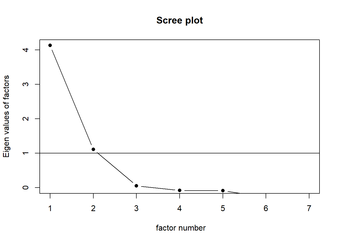

Two axes will be chosen to explain FA.

Realisation FA

fa.food <- factanal(food, factors = 2, rotation="varimax") #factor = 2 : number axis.
print(fa.food, digits=2, cutoff=.6, sort=TRUE)

## 
## Call:
## factanal(x = food, factors = 2, rotation = "varimax")
## 
## Uniquenesses:
##      bread vegetables     fruits       meat    poultry       milk       wine 
##       0.27       0.09       0.09       0.00       0.01       0.00       0.79 
## 
## Loadings:
##            Factor1 Factor2
## vegetables  0.75          
## fruits      0.93          
## meat        0.96          
## poultry     0.99          
## bread               0.85  
## milk                0.99  
## wine                      
## 
##                Factor1 Factor2
## SS loadings       3.55    2.20
## Proportion Var    0.51    0.31
## Cumulative Var    0.51    0.82
## 
## Test of the hypothesis that 2 factors are sufficient.
## The chi square statistic is 23.27 on 8 degrees of freedom.
## The p-value is 0.00303

library(psych)

loads <- fa.food$loadings

fa.diagram(loads)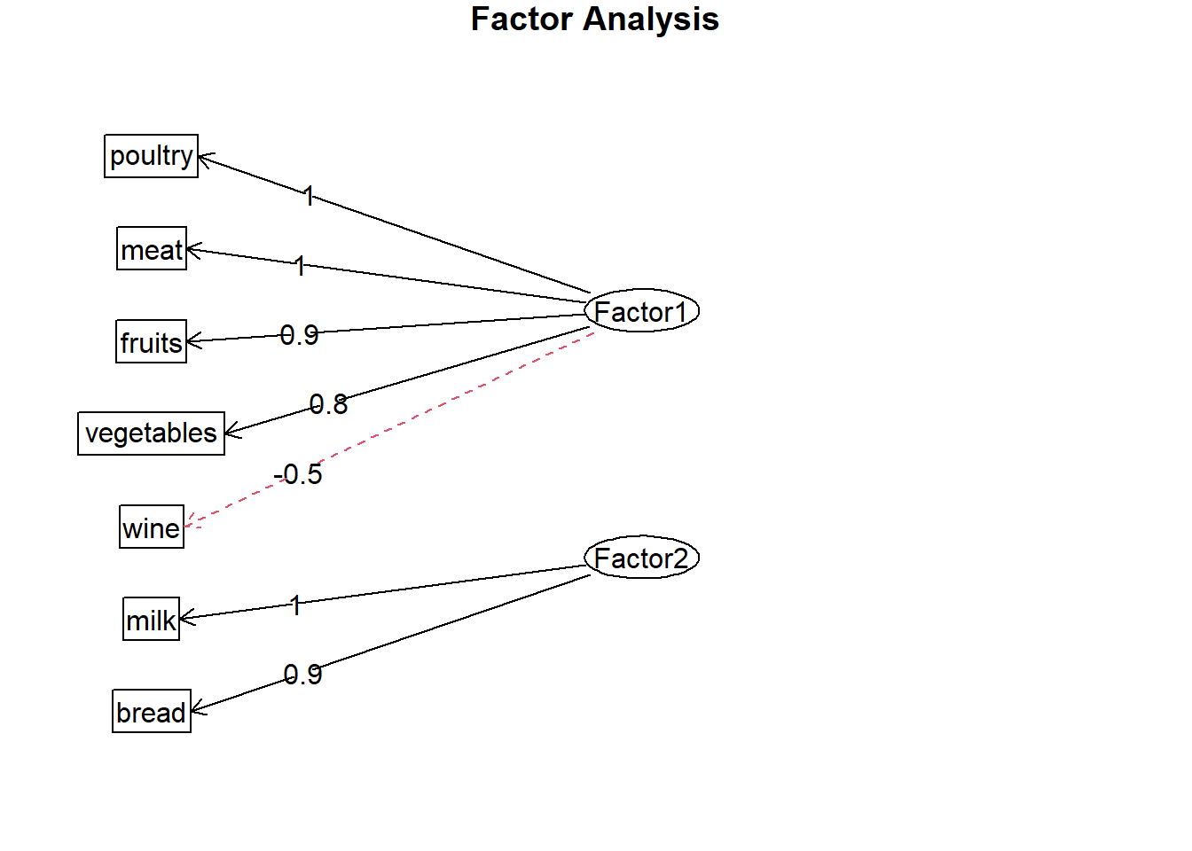

axis 1 : poultry / meat / fruits / vegetables / (wine..)

axis 2 : Milk / bread

load <- fa.food$loadings[,1:2] 
plot(load,type="n") 
text(load,labels=names(food),cex=.7)

lines(c(-1,1),c(0,0), lty = 3)
lines(c(0,0),c(-1,1), lty = 3)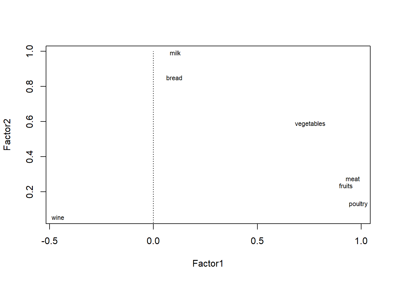

rbPal <- colorRampPalette(c('red','blue'))

loadings <- data.frame(fa.food$loadings[,1:2])

loadings$colF1 <- rbPal(20)[as.numeric(cut(loadings[,1],breaks = seq(-1,1,length = 20)))]
loadings$nam1 <- paste(row.names(loadings), round(loadings[,1], digits = 3), sep = "\n")
loadings$colF2 <- rbPal(20)[as.numeric(cut(loadings[,2],breaks = seq(-1,1,length = 20)))]
loadings$nam2 <- paste(row.names(loadings), round(loadings[,2], digits = 3), sep = "\n")


par(mfrow = c(2,1))
barplot(abs(loadings[,1]), col = loadings$colF1, ylim = c(0,1), ylab = "Factor 1", names.arg = loadings$nam1, cex.names = 0.8)
barplot(abs(loadings[,2]), col = loadings$colF2, ylim = c(0,1), ylab = "Factor 2", names.arg = loadings$nam2, cex.names = 0.8)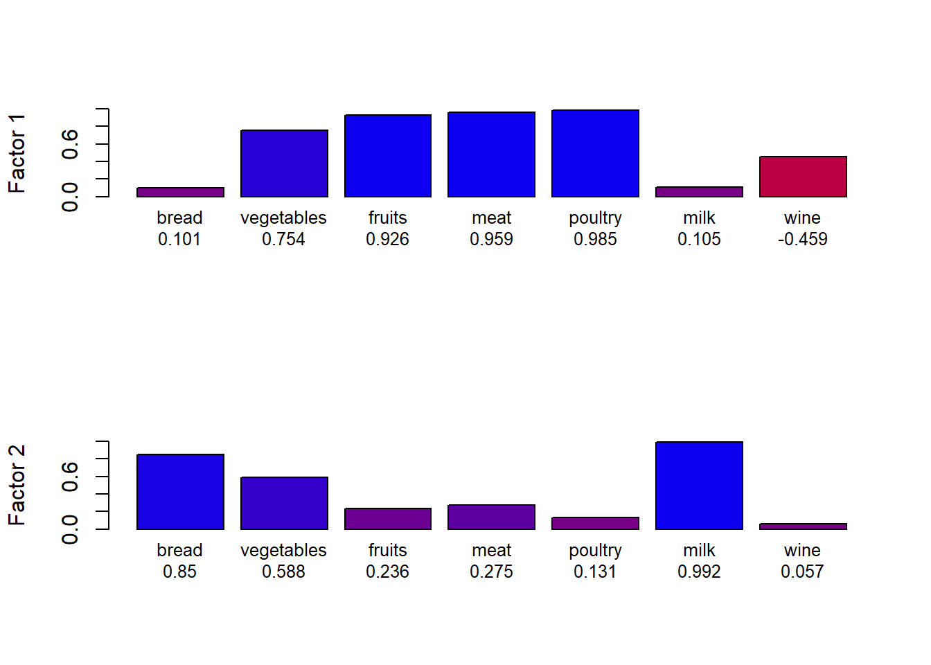

representation of each variable on each axis

round(fa.food$loadings, 3)

## 
## Loadings:
##            Factor1 Factor2
## bread       0.101   0.850 
## vegetables  0.754   0.588 
## fruits      0.926   0.236 
## meat        0.959   0.275 
## poultry     0.985   0.131 
## milk        0.105   0.992 
## wine       -0.459         
## 
##                Factor1 Factor2
## SS loadings      3.548   2.204
## Proportion Var   0.507   0.315
## Cumulative Var   0.507   0.822

Comparaison with PCA :

During the PCA we also noticed that it was necessary to keep just 2 axes.

Resultat :

res<-PCA(food, scale.unit = TRUE, ncp = 5, graph = F)
var <- get_pca_var(res)
corrplot(var$contrib, is.corr=FALSE)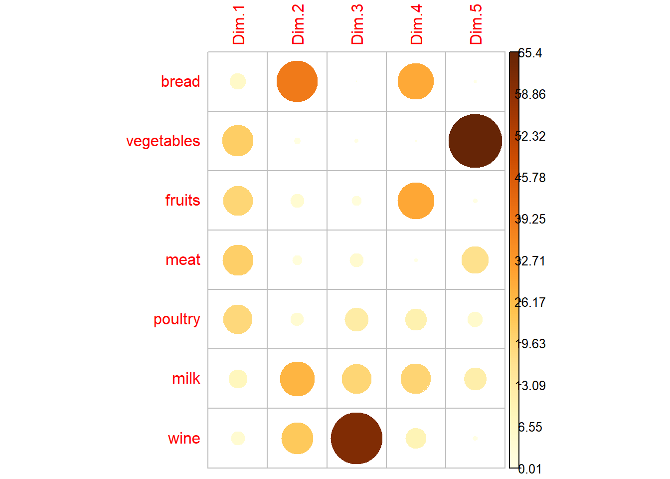

This graph shows that the important variables for each axis are the same for PCA and FA.